

The Billion-Parameter Problem
Fine-tuning a large language model (LLM) — that is, taking a pre-trained model and further training it on your own data so it picks up a new skill or style — is, for most people, a financial and logistical nightmare. A 70-billion-parameter model needs at least 140 gigabytes of VRAM (the memory on a graphics card) just to hold its weights, the numbers that encode what it has learned, in half-precision format. That's before training even starts.
Once you begin training, the memory demand balloons further. To update the model's behavior, you need to calculate a gradient for every one of those 70 billion parameters — a gradient is simply a measure of which direction each parameter should shift to reduce error. You also need to store the optimizer state, which is the running record your training process keeps of how each parameter has been changing, so it can decide the next adjustment. Between gradients and optimizer state, memory use can triple or quadruple, pushing the hardware requirement into the range of multi-million-dollar server clusters. For a solo developer, a researcher, or a small company, that cost is a non-starter. You're left using the model exactly as it was shipped, with no way to adapt it to your own needs.
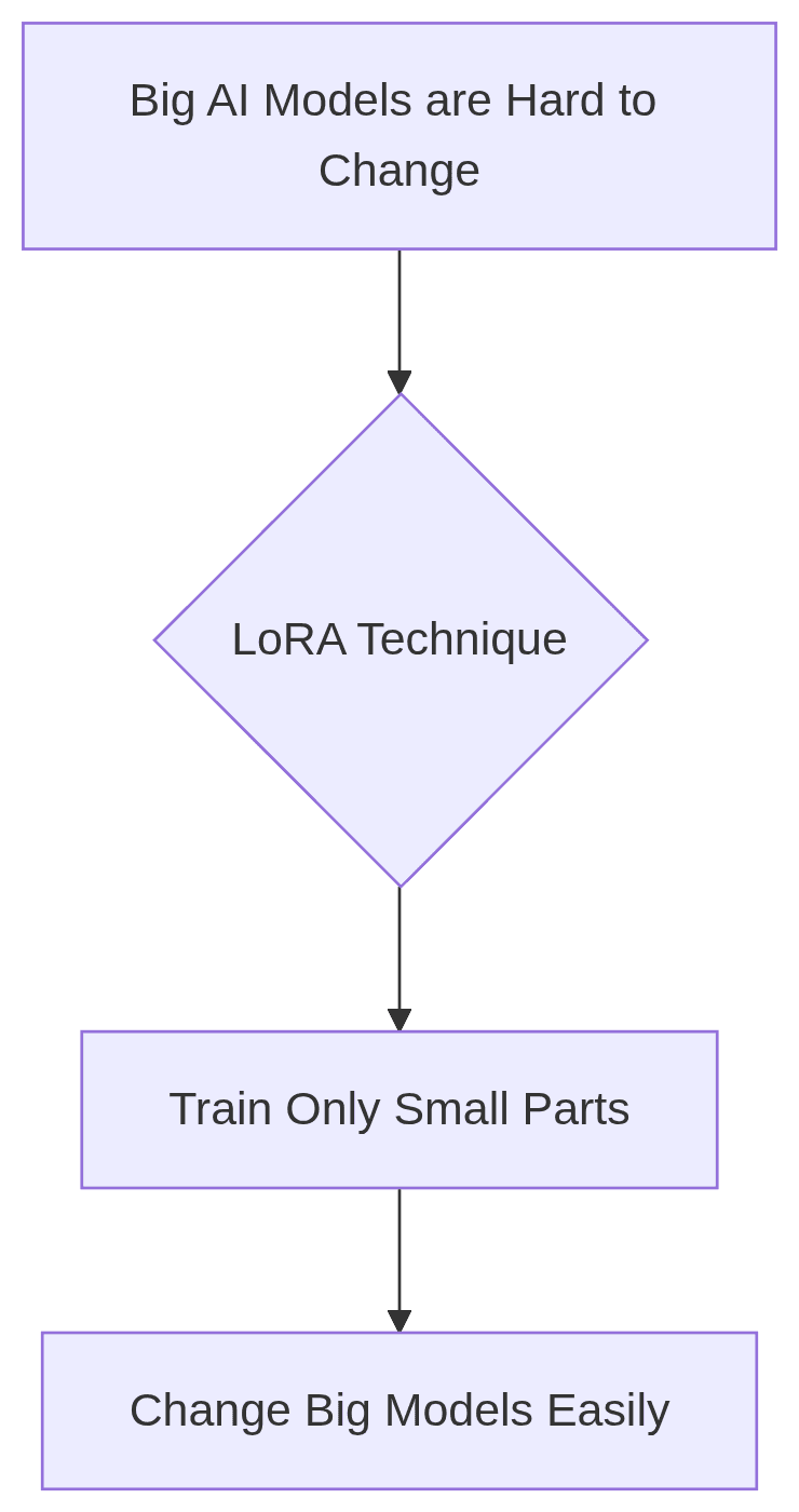
This is the problem that Low-Rank Adaptation, or LoRA, was designed to solve. It's a technique that makes fine-tuning large models dramatically cheaper. Instead of touching all of a model's parameters, LoRA locks (or "freezes") the vast majority of them in place and inserts a pair of small, trainable matrices — grids of numbers — into each layer of the network. By training only these small inserted matrices, which add up to a tiny fraction of the model's total size, you can adapt a huge model to a new task using a single, ordinary consumer-grade GPU. It's a big part of why LLM customization is no longer limited to organizations with massive compute budgets.
The Low-Rank Insight: How LoRA Works
The magic of LoRA comes from a key observation about how neural networks learn, introduced in the paper LoRA: Low-Rank Adaptation of Large Language Models ↗, which provides the mathematical and empirical foundation for the technique. The core idea is that the changes made to a model's weights during fine-tuning don't need to be complex.
Full Fine-Tuning vs. Adaptation
In a standard fine-tuning process, you start with a pre-trained weight matrix, let's call it W, and your training process learns an update, ΔW, to adjust it for your specific task. The new, fine-tuned weight matrix becomes W + ΔW. The problem is that ΔW is the same size as W. If W has a billion parameters, ΔW also has a billion parameters, and calculating it is the expensive part.
The authors of the LoRA paper hypothesized that this update matrix, ΔW, has a low “intrinsic rank.” In linear algebra, the rank of a matrix is a measure of its complexity—specifically, the number of linearly independent columns or rows. A low-rank matrix is simple; its information is highly redundant and can be compressed. LoRA leverages this by proposing that we don't need to compute the enormous ΔW directly. Instead, we can approximate it with two much smaller matrices.
The Rank Decomposition Trick
This is the central trick of LoRA: matrix decomposition. Any matrix can be approximated by multiplying two or more smaller matrices together. LoRA approximates the update ΔW with the product of two new matrices, B and A.
So, the update equation changes:
Full Fine-Tuning:
W_new = W_old + ΔWLoRA:
W_new = W_old + B * A
Here, W_old (the original pre-trained weights) is frozen and not trained at all. Only the new matrices, B and A, have their parameters updated during training.
Let's see why this is so powerful. Imagine W is a large 1000 x 2000 matrix. It has 2 million parameters. The update matrix ΔW would also have 2 million parameters to train.
With LoRA, we choose a small number for our rank, r. This rank r will be the shared dimension between our two new matrices. Let's pick r = 8.
Matrix
Awill have dimensions8 x 2000.Matrix
Bwill have dimensions1000 x 8.
When we multiply B * A (a 1000 x 8 matrix by an 8 x 2000 matrix), the result is a 1000 x 2000 matrix, exactly the same shape as ΔW. But how many parameters are we actually training?
Parameters in
A:8 * 2000 = 16,000Parameters in
B:1000 * 8 = 8,000Total Trainable Parameters:
16,000 + 8,000 = 24,000
We have replaced a 2,000,000-parameter training task with a 24,000-parameter one. That's a reduction of over 98%. This is why LoRA uses so little memory and compute. We are training less than 2% of the parameters we would have in a full fine-tune, but we still get a full-sized update matrix at the end.
A Worked Example: LoRA in Action
Let's make this more concrete by looking at a single weight matrix inside a Transformer's self-attention block. A common target for LoRA is the query projection matrix, W_q.
Suppose we have a model where the internal dimension (d_model) is 4096 and the head dimension (d_head) is 128. The query weight matrix W_q would have dimensions 4096 x 128.
Parameters in
W_q:4096 * 128 = 524,288
In a full fine-tune, we would need to store the gradients and optimizer state for all half-a-million of these parameters.
Now, let's apply LoRA. We'll choose a rank r = 8, a common starting point.
Freeze
W_q: The original 524,288 parameters are locked. They will not be updated during training.Create LoRA matrices:
Create matrix
Awith dimensionsr x d_head, which is8 x 128.Create matrix
Bwith dimensionsd_model x r, which is4096 x 8.
Calculate trainable parameters:
Parameters in
A:8 * 128 = 1,024Parameters in
B:4096 * 8 = 32,768Total trainable LoRA parameters:
1,024 + 32,768 = 33,792
For this one matrix, we've reduced the number of trainable parameters from 524,288 to just 33,792. That's a 93.5% reduction. When you apply this same logic to several weight matrices in each layer of a massive model, the savings become astronomical.
The Forward Pass Calculation
During training and inference, the model's computation changes slightly. A vector x passing through this layer is transformed like this:
output = x * W_q
With LoRA, the new calculation is:
output = x * (W_q + B * A)
For computational efficiency, this is rearranged using the distributive property:
output = (x * W_q) + (x * B * A)
This is a key detail. The first term, x * W_q, is a computation using the original, frozen, and highly optimized weights. The second term, (x * B * A), is the learned "correction" or "adjustment" from our LoRA adapter. The model computes the original path and then adds a small, learned deviation on top.
The Payoffs and the Trade-offs
The efficiency gains are just the beginning. The LoRA architecture provides several powerful operational advantages, but it also introduces new considerations.
The Big Win: Portable, Swappable Adapters
Because the original model is frozen, the result of a LoRA training run is not a new 140 GB model. It's just the small A and B matrices. These are often called a LoRA adapter, and they are tiny—typically a few megabytes to a few hundred megabytes, depending on the rank and which layers you adapt.
This has profound implications:
Portability: You can easily save, share, and load these adapters. Instead of sending a massive model checkpoint to a colleague, you can send a tiny adapter file.
Multi-tasking: You can fine-tune one base model for dozens of different tasks, resulting in dozens of small, specialized adapters. Want your LLM to be a Python expert? Train a Python adapter. Want it to adopt the persona of a cheerful pirate chatbot? Train a pirate adapter.
Dynamic Swapping: At inference time, you can load the single base model into GPU memory and dynamically apply different adapters on a per-request basis. A server can handle a request for code generation by loading the Python adapter, and the very next request for summarization by swapping in the summarization adapter, all without reloading the giant base model. This dramatically reduces operational complexity and cost for multi-tenant applications.
Avoiding Catastrophic Forgetting
When you fully fine-tune a model on a new, narrow task (e.g., medical terminology), it often gets worse at tasks it was previously good at (e.g., creative writing). This phenomenon is known as catastrophic forgetting. The model overwrites its general knowledge to specialize.
LoRA largely mitigates this. Since the original pre-trained weights W are frozen, the model's vast store of general knowledge is perfectly preserved. The LoRA adapter B * A only learns to add or subtract from the existing behavior. It's a non-destructive process. If you don't like the adapter's performance, you can simply detach it, and the model reverts to its original, pristine state.
What's the Catch? Choosing Your Rank
LoRA isn't a magic wand; it introduces a new hyperparameter to tune: the rank, r. The rank determines the expressivity and capacity of your adapter. It's a direct trade-off.
Low Rank (e.g., 4, 8, 16): This results in the smallest, fastest-training adapters. It's ideal for simpler adaptations, like tweaking a model's style or tone. However, if the rank is too low for the complexity of the task, the model may underfit and fail to learn the desired behavior adequately.
High Rank (e.g., 64, 128, 256): This gives the adapter more parameters and more capacity to learn complex patterns. It can be necessary for more demanding tasks that require learning new facts or skills. The downsides are that training is slower, the adapter file is larger, and you run a higher risk of overfitting to your fine-tuning data, making the adapter less general.
Choosing the right rank is an empirical process. It's often best to start small (e.g., r=8 or r=16) and increase the rank only if performance is not satisfactory.
When Not to Use LoRA
LoRA is exceptionally good at adapting a model's existing knowledge to a new domain or style. It is less effective when a task requires the model to learn a large body of entirely new information that is not represented in its pre-training data.
For example, if you want to teach a general-purpose LLM the entire contents of a proprietary, highly technical internal knowledge base, a low-rank update might not have enough capacity. In such cases, more intensive methods like full fine-tuning or even continued pre-training on the new corpus might be necessary. LoRA is a scalpel for precise adjustments, not a sledgehammer for wholesale reconstruction.
Getting Started with LoRA
The good news is that you don't have to implement the matrix multiplication hooks yourself. The AI/ML ecosystem has embraced LoRA, and it is now a standard feature in popular open-source libraries like Hugging Face's transformers and peft (Parameter-Efficient Fine-Tuning).
Implementing LoRA conceptually follows a few simple steps, as shown in this pseudo-code:
# 1. Load your pre-trained base model
# This is the large, frozen part of your system.
model = load_pretrained_model("big-model-name")

# 2. Define a LoRA configuration
# This tells the library where and how to apply the adapters.
lora_config = {
    "r": 16,  # The rank of the update matrices.
    "lora_alpha": 32, # A scaling factor, often set to 2 * r.
    "target_modules": ["q_proj", "v_proj"], # Which layers to adapt.
    "lora_dropout": 0.1, # Dropout for regularization.
}

# 3. Create a model ready for parameter-efficient training
# The library wraps the original model, adding the adapters.
lora_model = apply_lora(model, lora_config)
# Print the trainable parameters to confirm the massive reduction.
print_trainable_parameters(lora_model)

# 4. Train the model as usual
# The library ensures that only the LoRA adapter weights are updated.
train(lora_model, your_dataset)

# 5. Save the result
# This saves only the tiny adapter weights, not the entire model.
lora_model.save_adapter("./my-custom-task-adapter")
The lora_alpha parameter is a scaling factor applied to the update. The effective update becomes (alpha / r) * B * A. This helps balance the influence of the initial weights and the new adapter weights, often stabilizing training, especially when changing the rank r. A common heuristic is to set alpha to twice the rank r.
The Future is Efficient
What LoRA actually changes is the unit of work. Instead of shipping a full 140 GB model every time you want a new behavior, you ship a file that might be a few megabytes to a few hundred megabytes — small enough to email, version in a code repository, or store dozens of copies of on a single machine. A team building a customer support bot, a coding assistant, and a document summarizer no longer needs three fine-tuned copies of a 70B model sitting in storage and competing for GPU memory; it can keep one frozen base model loaded and swap adapters in and out per request.
That doesn't remove every hard choice. You still have to pick a rank, and it's easy to get wrong in either direction: too low, and the adapter can't learn the task; too high, and you lose some of the speed and memory advantage while risking overfitting to your training data. You still have to decide, task by task, whether LoRA's scalpel is the right tool at all — teaching a model an entirely new body of facts it never saw in pre-training is a job better suited to full fine-tuning or continued pre-training on that data, not to a low-rank adapter. And because the base model is never touched, LoRA is a good fit for correcting or steering behavior, but a poor fit for anyone hoping to overwrite a model's core knowledge outright.
What it does deliver, reliably, is a lower floor for entry: an approach where adapting a 70-billion-parameter model to a specific task is a job for one GPU and a modest training run, not a data center.