

Giant Prodigies Who Left School Too Early
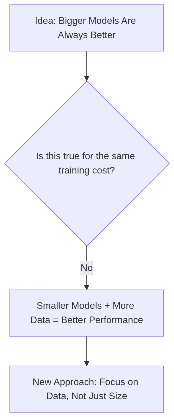
In March 2022, a team at DeepMind trained more than 400 language models to test an assumption the whole field had been building on for years: that bigger is always better. A large language model, or LLM, is a program trained to predict and generate text, and its "size" is usually described by its parameter count — the number of tunable internal values that store what it has learned. The recipe for making one better had always seemed obvious: add more layers, more attention heads (the parts of the model that let it weigh different words against each other), and more billions of parameters.
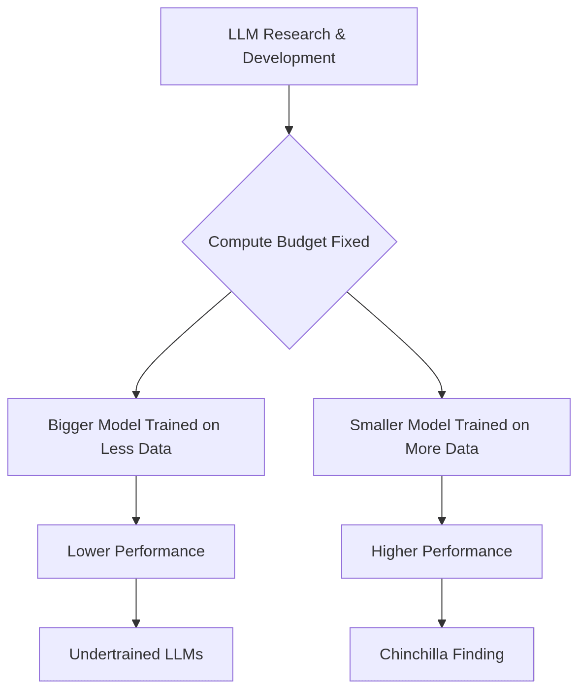
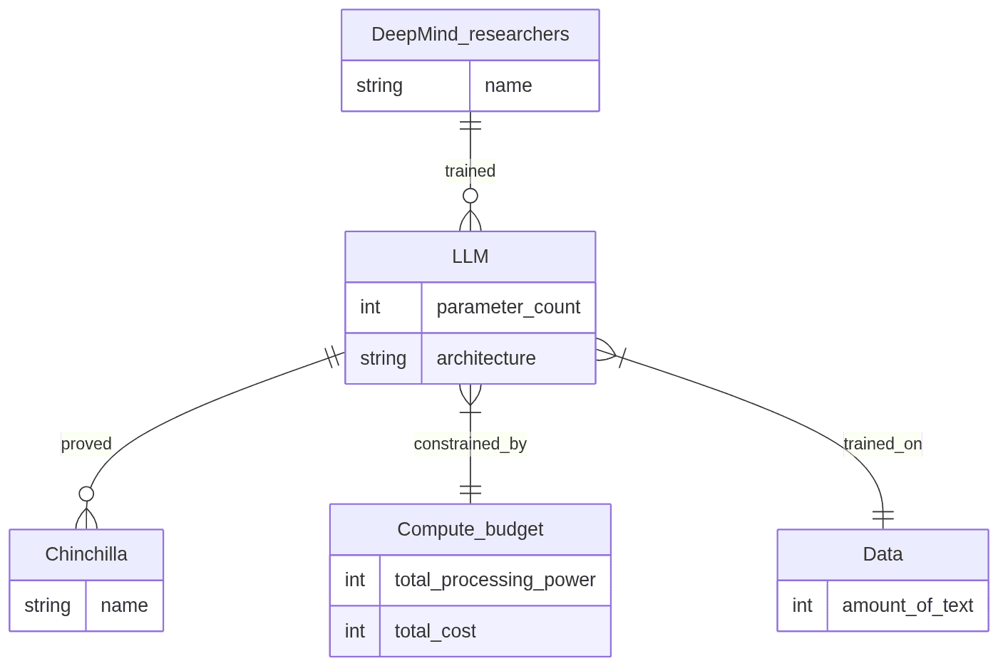
That recipe worked, but it was ferociously expensive, and it turned out to rest on a mistake. The DeepMind researchers looked at what happens when you fix your compute budget — the total amount of processing power, and therefore money, you're willing to spend on training a model — and asked a simple question: for that fixed budget, is the biggest model you can afford really the smartest choice? The answer was no. A smaller model trained on far more text consistently beat a larger model trained on less, for the exact same cost. This became known as the "Chinchilla" finding, after the model the researchers built to prove it, and it was a quiet revolution. It showed that many of the era's flagship models were, in effect, prodigies pulled out of school too soon — built with enormous capacity to learn, but never fed enough material to fill it. Researchers call this being "undertrained."
The Tyranny of Scale
Before 2022, a clear trend dominated LLM research and development: landmark models were celebrated primarily for their size. The prevailing wisdom, backed by early scaling laws, held that performance scaled predictably with parameter count, so the path to a better model was simply to build one with more of them.
This led to an arms race, with labs and companies pouring astronomical resources into training models with ever-higher parameter counts. The working assumption was that a model's capacity to learn complex patterns, nuances, and facts about the world was primarily a function of its size. Data was, of course, essential, but the focus stayed on scaling the neural network architecture itself.
This "bigger is better" philosophy created a few practical problems:
Astronomical Training Costs: Training a model with hundreds of billions of parameters requires thousands of high-end GPUs running for weeks or months, costing millions of dollars in electricity and hardware.
Crippling Inference Costs: Even after a model is trained, running it is expensive. The number of parameters directly impacts the memory and computation required for every single prediction. Larger models are slower and costlier to serve, making them impractical for many real-world applications.
A Point of Diminishing Returns: While performance improved with size, it wasn't always clear if the gains justified the exponential increase in cost. Was a model with 500 billion parameters truly twice as good as one with 250 billion, or just marginally better at a few tasks while being ten times more expensive to run?
The industry was scaling up model size because it was the most obvious knob to turn. But it was only one of three critical variables — the other two, the amount of training data and the total compute budget, were about to take center stage.
Introducing Compute-Optimal Scaling
To understand the shift, we need to talk about scaling laws — not laws of nature, but empirical formulas that researchers derive to predict a model's performance without having to fully train it first.
What are Scaling Laws?
A scaling law in machine learning is a mathematical relationship that connects a model's final performance (usually measured by its "loss," where lower is better) to the resources used to create it. For LLMs, the three key resources are:
Compute (C): The total number of floating-point operations (FLOPs) used for training. This is your total budget.
Model Size (N): The number of parameters in the model.
Data Size (D): The number of tokens (pieces of words) in the training dataset.
The total compute C is roughly proportional to the product of the model size N and the data size D. That is, C ≈ 6 * N * D. The 6 comes from the fact that for each token processed by a standard transformer model, there is one forward pass (costing 2 * N FLOPs) and one backward pass (costing 4 * N FLOPs).
The goal of scaling law research is to find the function L(N, D) that predicts the final loss L for a model of size N trained on D tokens. If you have this function, you can work backward. Given a fixed compute budget C, you can figure out the ideal combination of N and D that will give you the lowest possible loss. This is called compute-optimal training.
The Chinchilla Bombshell
In March 2022, a team of DeepMind researchers published a paper that re-examined the scaling laws for LLMs: Training Compute-Optimal Large Language Models ↗.
Previous work had suggested that to improve performance, model size (N) should grow faster than the training dataset size (D). The DeepMind team decided to test this rigorously. They trained over 400 models, systematically varying the model size from 70 million to over 16 billion parameters, and the data size from 5 billion to 500 billion tokens.
By carefully fitting a new scaling law to this mountain of experimental data, they arrived at a startling conclusion. For a fixed compute budget, the previous generation of LLMs was incorrectly proportioned. The researchers found that for optimal performance, the model size and the training dataset size should be scaled in roughly equal proportion. If you double the model size, you should also double the number of training tokens.
This meant that for any given massive model of the era, a much smaller model trained on significantly more data could achieve a better score while using the exact same amount of training compute. This smaller, compute-equivalent model was named Chinchilla. It was proof that the industry had been building models that were too big and feeding them too little.
One Budget, Two Models: A Worked Example
Let's make this concrete. Imagine you are a project lead in 2021 with a fixed, massive compute budget — let's call it C_budget. You want to train the best possible LLM. Based on the prevailing wisdom, you decide to build a very large model.
The "Goliath" Approach (Pre-Chinchilla):
Model Size (N): You allocate most of your budget to parameters, creating a massive 280-billion parameter model.
Data Size (D): With the remaining budget, you can afford to train this model on a dataset of 500 billion tokens.
The total compute cost is proportional to 280B * 500B. This model is huge, and it performs well, setting new benchmarks. You've succeeded by the standards of the day.
Now, let's step into the shoes of the DeepMind researchers. They have the exact same compute budget, C_budget. But they use their new, compute-optimal recipe.
The "David" Approach (Chinchilla-Optimal):
Model Size (N): They build a much smaller model, only 70 billion parameters (one-fourth the size of Goliath).
Data Size (D): Because the model is smaller, they can afford to train it on a much larger dataset for the same total cost. They use a dataset of 1.4 trillion tokens (almost three times more data).
The total compute cost is proportional to 70B * 1.4T, which is roughly the same as the Goliath model's training cost.
When both models finish training, the results are stunning. The 70-billion parameter Chinchilla model, despite being four times smaller, outperforms the 280-billion parameter "Goliath" model on a wide range of downstream evaluation benchmarks. It has a lower loss, meaning it is fundamentally better at predicting the next token. It is, in essence, "smarter" and more capable, all because it was trained on a dataset that was appropriately sized for its learning capacity.
This is the core of the Chinchilla finding: for the same price, a smaller, better-educated model beats a larger, undertrained one.
Why a Smaller, Better-Trained Model Wins
The implications of this discovery were immediate and profound. It wasn't just an academic curiosity; it changed the economics and strategy of building and using LLMs.
Lower Inference Cost
This is the most direct and impactful benefit. The cost and latency of getting a response from an LLM are directly proportional to its parameter count.
The 70B Chinchilla-style model is 4x cheaper and 4x faster to run than the 280B Goliath-style model.
It requires one-fourth of the expensive GPU memory to host.
For any application that calls an LLM frequently, this difference is enormous — a product that was economically unviable with the larger model could become profitable with the smaller, more capable one, delivering better performance for a fraction of the operational cost.
Better Fine-Tuning and Downstream Performance
A model's final loss after pre-training is a strong indicator of its quality. A lower loss means the model has developed a more accurate and robust internal representation of language. When you take a pre-trained model and fine-tune it for a specific task like document summarization or code generation, you are starting from that internal representation.
The Chinchilla-optimal model, having been trained to a lower loss, provides a superior foundation. It has seen more examples of the world's text, allowing it to learn more generalizable patterns. When you fine-tune it, it adapts more quickly and reaches a higher peak performance on your specific task. The undertrained larger model, by contrast, may have more raw capacity, but much of it is "unfilled." Its understanding is less refined, making it a poorer starting point.
The End of "Bigger is Always Better"
The Chinchilla paper effectively ended the era where parameter count was the sole metric of progress. It introduced a more sophisticated question: "Is this model well-trained for its size?"
The new goal wasn't just to build the biggest possible model, but to assemble the largest high-quality dataset and then build a model of the corresponding optimal size. The bottleneck had shifted from architecture to data. This forced a massive industry-wide investment in data sourcing, cleaning, and curation.
How to Think About Model Scaling in 2026
Four years on, the Chinchilla lessons have been thoroughly absorbed by the industry, and they're worth turning into habits rather than history. Today, no serious practitioner judges a model on its parameter count alone. Here's how to put that into practice.
When Choosing a Foundation Model:
Don't be seduced by the largest parameter count on the spec sheet. When a new model is released, the two numbers you should look for side by side are the parameter count and the training token count — how much text it was actually trained on.
As a rule of thumb, look for a ratio of roughly 20 tokens of training data for every parameter in the model. For example:
A 70-billion parameter model should be trained on at least
70B * 20 = 1.4Ttokens.A 13-billion parameter model should be trained on at least
13B * 20 = 260Btokens.
A model that falls well short of this ratio — a large parameter count paired with a comparatively small training set — is likely a "Goliath": an undertrained model built on pre-Chinchilla assumptions. In practice, it will probably cost more to run and perform worse than a smaller, properly-trained alternative, so it's worth checking this ratio before committing to a model for a product.
When Training Your Own Model:
If you are in the fortunate position of training a model from scratch, the Chinchilla scaling laws give you a clear playbook.
Start with your compute budget. How many GPU-hours can you afford? This is your
C_budget.Estimate your data budget. How much high-quality training data can you realistically acquire and clean? This gives you
D.Calculate the optimal model size. Using the
C ≈ 6 * N * Dformula, you can determine the optimal parameter countNfor your compute and data budget.
Resist the temptation to build a model that's too large for your dataset. Every dollar spent on extra parameters that your data can't feed is a dollar wasted — you'll get a better final model by training a smaller architecture for more steps on more data than by inflating parameter count and starving it of examples.
What the Chinchilla paper leaves open is where the next bottleneck sits. It solved the problem of proportion — how big a model should be relative to its data — but it assumed high-quality data was there for the taking. As datasets have grown toward the size of the readily available text on the internet, the harder question has become where the next trillion good tokens come from, and whether the same 20-tokens-per-parameter ratio still holds once you run low on new material to feed the model. The race for scale hasn't ended; it has simply become a race for scale in both data and parameters, run under the discipline of compute-optimality rather than the old instinct to just build bigger.